
Tau Boo First Run
“Awesome detection of the planet around the star Tau Boo! That is truly ‘spectracular’!”
Geoff Marcy
In February of 2000 we took our telescope and spectrograph to Arizona with the goal of detecting the known extrasolar planet around the star tau Boo. After a three week struggle with bad weather and a defective grating, we came up with enough data to resolve the planets orbit. The plots below show the data in various configurations from this run. We believe this was the first radial velocity detection of an extrasolar planet by amateurs.
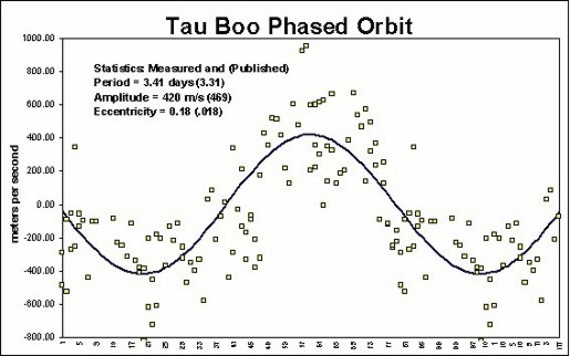
Above is the combined data points phased into a single orbit. The dark line represents the original orbit from Marcy and Butler.
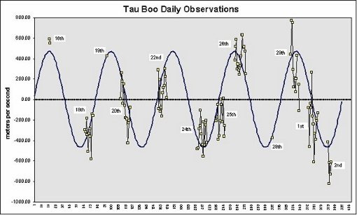
This shows the daily observations for the run. The sine wave is plotted from the published orbit data and is only lined up visually to our data. We were hampered by continuous bad weather and aberrations that required us to block half the grating. A good night produced about 13 exposures of 25 minutes each. We shot at every possible opportunity, quite often through thin clouds, thus some nights only produced a few good S/N exposures. The data shown has Earth’s diurnal and orbital motion subtracted via IRAF. It became obvious after a few days that we were seeing variations in the star’s velocity.
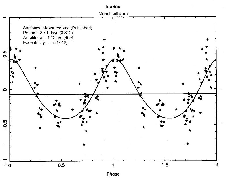
This is a printout from Caty Pilachowski at NOAO who independently used MONET software to fit the best orbit to our data. The software produces a sine wave from a “best fit” solution. The resulting numbers agree very well with Marcy and Butler’s published data. Our orbit is more eccentric than published, but we attribute this to lack of data at the negative peak in the orbit. We would like to thank Caty for helping us out with this analysis.
Measured and (Published)
Period = 3.17 days (3.312)
Amplitude = 390 m/s (469)
RMS = 210 m/s
Mean = -0.6 m/s
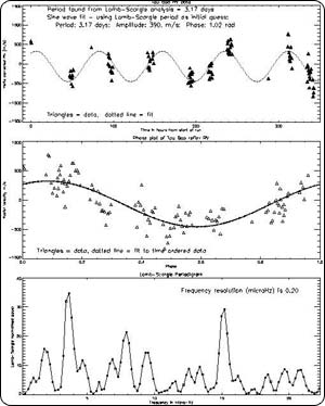
This is the second independent evaluation done by professional astronomer John Innis in Tasmania. He used the Lomb-Scargle routine in IDL to determine the most significant periodicity in the data (=3.2 days), and then used this as input into a least-squares sine wave fit to produce the fitted curve shown. Here we see the data plotted as daily observations with the best fit sine wave in the top box. The middle box holds the data phased about a single orbit. The lower box is a power spectrum which shows a strong peak at the frequency most represented in the data. We have never met John but want to thank him for taking an interest in amateur astronomy halfway around the world.
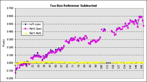
This graph shows the spectrum shift after the reference position has been subtracted. The continuous upward trend in the purple data is from Earth’s diurnal and orbital motion. The yellow dots are the result of subtracting the first reference fiber from the second reference. If the system is stable, this plot should hover around zero, which it does.
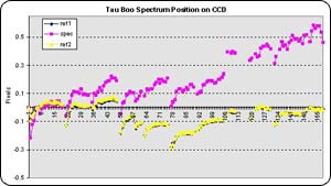
This shows the unprocessed positions of the different spectrums on the CCD. There are non-random trends in the reference spectrums from each night’s startup which are minimized by running test exposures for several hours before the run.
More than two years ago we set out to answer the question, “Can amateur equipment detect an extrasolar planet?” We hope we have answered that question to everyone’s satisfaction. We are now ready to start on our second question, “Can amateur equipment DISCOVER an extrasolar planet?”
We would especially like to thank the professional astronomers Don Barry, John Innis, Caty Pilachowski and Mark Trueblood who have helped with this project.